
NLP: Twitter Sentiment Analysis (2): Perform Exploratory Data Analysis
- Sep 8, 2023
- 3 min read
Updated: Sep 13, 2023

Welcome to NLP: Twitter Sentiment Analysis (2)!
Project summary:
In this series, NLP: Twitter Sentiment Analysis, we're going to train a Naive Bayes classifier to predict sentiment from thousands of Twitter tweets.
This project could be practically used by any company with social media presence to automatically predict customer's sentiment (i.e.: whether their customers are happy or not).
The process could be done automatically without having humans manually review thousands of tweets and customer reviews.
Let's go.
1. Create heatmap
Use seaborn to create heatmap showing the distribution of the tweets that is null:
sns.heatmap(tweets_df.isnull(), yticklabels = False, cbar = False, cmap="Blues")▲ sns calls seaborn library to perform heatmap function to generate a heatmap.
tweets_df.isnull() defines the data showing on the heatmap is the count of tweets that is null, which has no content.
yticklabels = False means no y-axis label is showing.
cbar = False controls the color bar to be invisible on the heatmap.
cmap="Blues" defines the color of the heatmap to be blue.

(Result)
▲ If you find the result is an empty heatmap, don't worry. It's because our tweets data does not contain any null item. You're doing correctly!
2. Plot histogram
Create a histogram that showing the count of tweets with label 0 or 1 in red color.
tweets_df.hist(bins = 30, figsize = (13,5), color = 'r')▲ tweets_df calls pandas function hist() to generate a histogram.
bins sets the number of bars, the more bars, the thinner each bar is.
figsize defines the size of the histogram in term of inches for a (width, height) format.
color now sets as 'r', means red.

(Result)
3. Create countplot
Use seaborn to make a countplot showing the count of tweets with label 0 or 1:
sns.countplot(tweets_df['label'], label = "Count")▲ sns calls seaborn library to perform countplot function to generate a countplot.
tweets_df['label'] is the data to plot counts for, it's the label column of the tweets file.
label = "Count" is the label text of the y-axis.

(Result)
4. Get length of each tweets
Create a new column "length" to get the length of each tweet:
tweets_df['length'] = tweets_df['tweet'].apply(len)▲ tweets_df['length'] creates a new column 'length'.
We use tweets_df['tweet'] column to call apply(len) function to generate a new column length, which contains the length of each tweet.
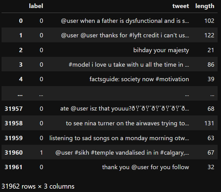
(Result)
Then, when you type the following command, you'll see the updated statistics for the length column:
tweets_df.describe()
(Result)
5. View the shortest tweet
From the statistics above, we knew that the shortest tweet has a length of 11, so here we get that message using 11 as a searching criteria:
tweets_df[tweets_df['length'] == 11]['tweet'].iloc[0]▲ tweets_df[tweets_df['length'] == 11] creates a new dataframe showing only the rows that the length column has a value of 11.
['tweet'] means showing only the value in the tweet column.
iloc[0] means show only the text content of the tweet without any additional information.
Although the length states '11', it includes the blank space.

(Result)
▲ Surprise, the shortest tweet is a very sweet message!
6. Alternative to plot histogram
Apart from tweets_df.hist(bins = 30, figsize = (13,5), color = 'r'), there's another way to create histogram:
tweets_df['length'].plot(bins = 100, kind = 'hist')▲ tweets_df calls pandas function plot() to generate a plot.
bins sets the number of bars, the more bars, the thinner each bar is.
So in this case, bins = 100 is much thinner than bins = 30.
kind now sets as 'hist', means the plot type would be histogram.

(Result)
Congratulations on completing this tutorial!
Never hesitate to seek further knowledge or ask questions.
See you in NLP: Twitter Sentiment Analysis (3)!
© 2023 Harmony Pang. All rights reserved.

Comments